

In Part 1 we showed that inference efficiency is no longer captured by simple tokens-per-second on a single GPU. Modern workloads introduce variable reasoning depth, prefill/decode disaggregation, aggressive KV cache reuse and compression, and contention across heterogeneous hardware tiers. The measurement model has moved from isolated benchmarks to end-to-end production systems.
Traditional lab benchmarks are still useful for regression and ceilings, but they lack the representative workload patterns to predict real cost and performance under mixed, stateful traffic.
The Benchmark Illusion
Classic benchmarks follow a clean pattern: load a model, warm caches, issue one prompt on an isolated GPU, and record TTFT, TPOT, and tokens/second. These numbers are repeatable and easy to compare.
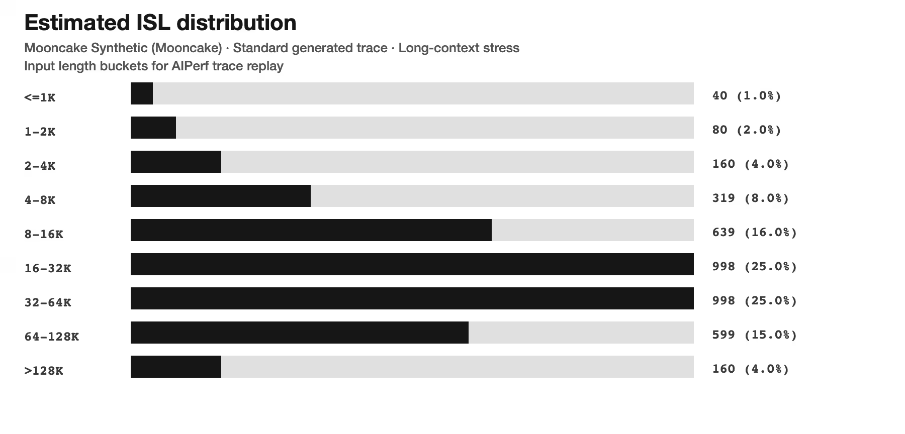
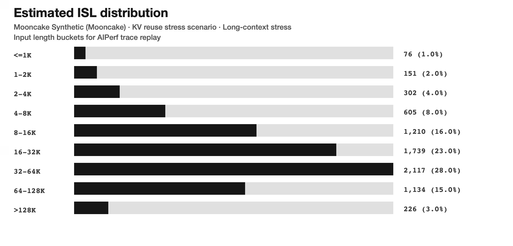
They also hide the behaviors that dominate production economics. Real inference is a continuous interleaved stream. We see a variety of short prompts competing with long-context RAG, agentic loops that repeatedly hit the same context (NVIDIA reports 85–97% reuse for coding agents), and reasoning models that can emit 10K–20K hidden tokens before a final answer.
Each hidden token is a full forward pass. All requests fight for the same HBM. The relevant metric is no longer peak throughput on a warm cache. It is effective cost per successful output under realistic contention, reuse patterns, and tiered storage.
Production-Sourced Interleaved Traces
The foundation of credible measurement is replayable traces captured from production or high-fidelity staging. The metrics must reflect the true diversity and unpredictability of enterprise inference workloads.
Essential trace fields to do this must include:
- Request timing (arrival, prefill start/end, decode start/end, completion)
- Token counts (input, visible output, hidden reasoning)
- Context profile (length, reuse overlap, retrieved documents, agent/tool loops)
- Cache events (hit/miss per tier, size, age, eviction, retrieval latency)
- Phase placement and KV handoff (especially under disaggregation)
- Resource counters (HBM pressure, network transfer, flash/storage I/O, power)
- Outcome (success, quality gate, retry, cancellation)
A good trace lets you replay the exact workload mix against different serving policies, cache configurations, hardware pools, or storage tiers while holding the input constant. This turns benchmarking into controlled experimentation rather than guesswork.
Useful Lab Baselines (in Context)
Production traces complement, rather than replace, controlled baselines:
- Warmup/query ceiling – Best-case model + serving stack behavior. Useful for regression and upper bounds.
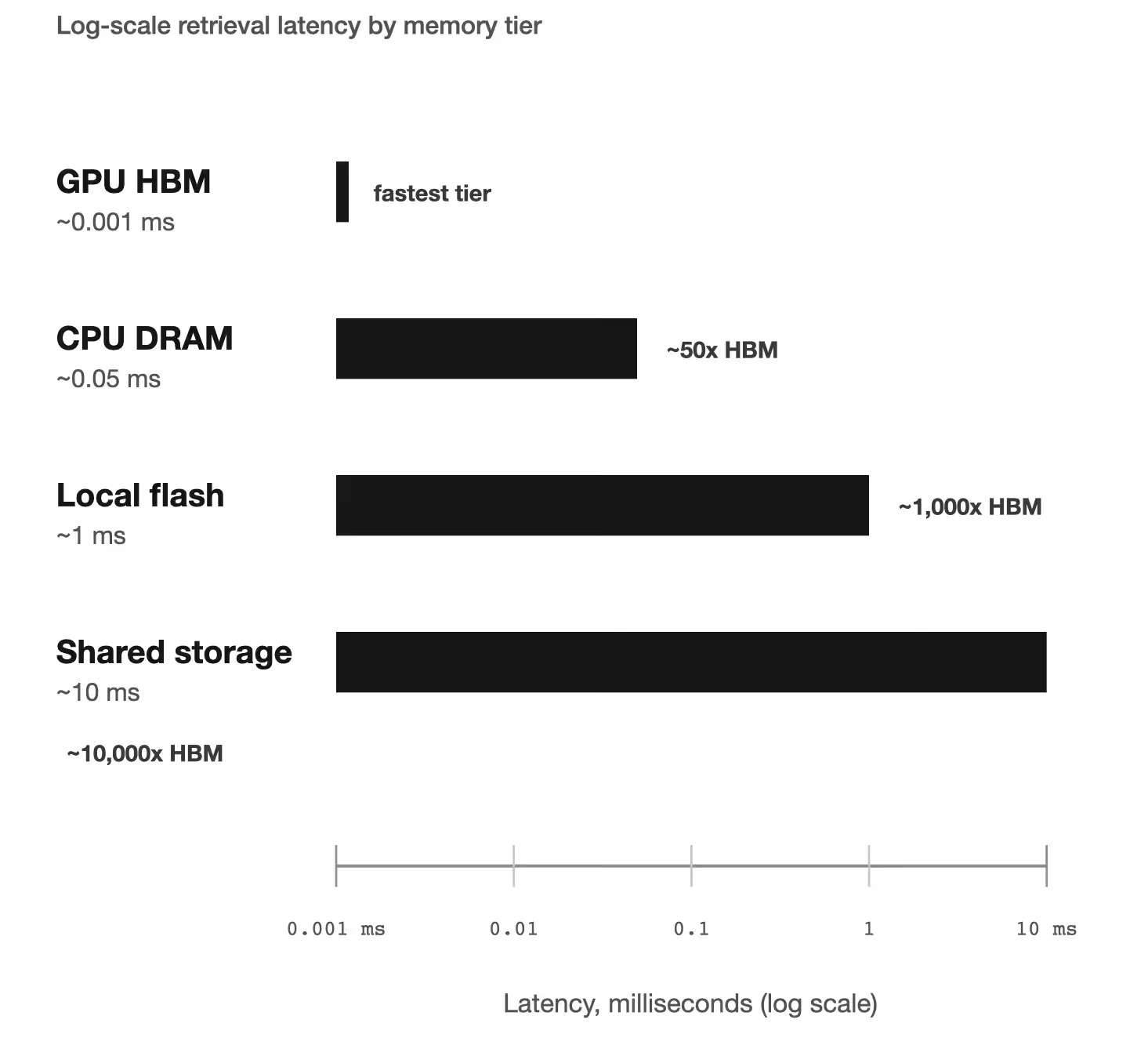
- Recompute upper bound – Cost of regenerating KV state. Defines the “retrieve must beat this” threshold.
- Prefill/decode isolation – Measures each phase independently (compute-bound prefill vs. memory-bound decode) and the cost of KV transfer under disaggregation.
The error is treating any single baseline as representative. A warm-cache run hides contention; a recompute test ignores reuse; isolated phases miss handoff overhead.
Effective Efficiency Metrics
A practical north-star metric is an effective efficiency across every element:
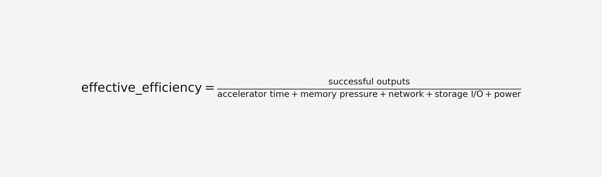
Track it per dollar and per watt, broken down by workload class. Supporting metrics that explain movement include:
- Tiered cache hit rates (HBM, DRAM, flash, shared storage)
- Retrieve-versus-recompute breakeven points per context length and tier
- Reasoning depth multiplier (hidden tokens per visible answer)
- Prefill/decode split efficiency and KV handoff cost
- Compression impact (memory savings vs. decompression overhead and quality)
| Metric | Synthetic Typical | Production Range | Key Insight |
|---|---|---|---|
| Cache hit rate (overall) | 90–95% | 60–85% (highly variable) | Contention and cold starts dominate |
| TTFT under load | <0.5 s | 1–5+ s | Queueing and misses matter |
| Effective tokens/$ | High | 30–70% of peak | Goodput > raw throughput |
| Hidden reasoning multiplier | ~1× | 5–50×+ for agentic | Dominant cost driver |
Practical Benchmarking Workflow
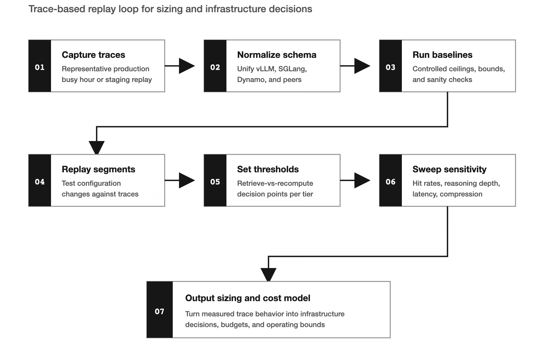
The benchmarking workflows must be consistent to allow for iteration, tuning, and comparisons. These are the steps that are being used to create and test truly representative inference traces:
- Capture representative production traces (busy hour or staging replay).
- Normalize schema across frameworks (vLLM, SGLang, Dynamo, etc.).
- Run controlled baselines for ceilings and bounds.
- Replay trace segments against configuration changes.
- Determine retrieve-vs-recompute thresholds per tier.
- Perform sensitivity sweeps (hit rates, reasoning depth, network latency, compression).
- Output a sizing and cost model that supports infrastructure decisions.
Implications for AI Infrastructure
It is only through accurate measurement that KV cache management, tiered storage, and fast retrieval are revealed as first-order concerns. When prefill and decode are disaggregated, KV state becomes a distributed object. When agentic workloads dominate, cache locality becomes an economic lever. When reasoning depth varies, cost per query is no longer visible from the final answer.
Next: The Multivariate Model
In Part 3 we will map out the full set of variables and equations, with examples for cluster sizing, cache policy trade-offs, and cost forecasting under enterprise agentic workloads. Inference efficiency is difficult precisely because real systems are complex. Once you measure the actual system, optimization becomes engineering again.
Measuring Inference Efficiency Series: Part 1
AI inference efficiency in production measures effective cost and performance under real-world conditions (including variable reasoning depth, KV cache reuse, contention, and tiered storage) rather than isolated tokens-per-second on a warm cache.
Classic benchmarks use clean, isolated prompts and ignore production realities like interleaved traffic, agentic loops with high context reuse, hidden reasoning tokens (5–50×+ multiplier), and KV cache pressure across heterogeneous hardware.
KV cache management is a first-order concern. With high reuse rates (e.g., 85–97% in coding agents) and disaggregated prefill/decode, tiered storage (HBM → DRAM → flash) and intelligent retrieval-versus-recompute decisions directly impact latency, throughput, and cost.
Key metrics include tiered cache hit rates, effective tokens per dollar/watt, reasoning depth multiplier, TTFT under load, retrieve-vs-recompute breakeven points, and hidden reasoning costs—tracked against realistic production traces.
High-performance, intelligent storage with fast I/O, parallel file systems, and tiering accelerates KV cache retrieval, checkpointing, and data pipelines, reducing recompute overhead and enabling efficient production inference for enterprise workloads.