
Collaboration by DDN and NVIDIA
Key result: 1 billion vectors indexed in 6 hours
Why this benchmark mattersTogether, DDN and NVIDIA have demonstrated Milvus with AiSAQ on DDN Infinia at billion-vector scale, while maintaining production-grade recall and latency. What impressed me most was how well Infinia handled this workload on shared storage—serving a billion-vector index in place at 98% recall, while keeping tail latency consistent as we added more concurrent user requests. Combined with NVIDIA cuVS and GPU-accelerated index builds, we’re able to reduce indexing times from days to hours. This gives us a proven, high-density architecture for scaling RAG and other retrieval-intensive AI workloads.
Corey J. NoletDistinguished Engineer, Unstructured Data Processing, NVIDIA
Any Retrieval Augmented Generation (RAG) or similarity search system over growing datasets will eventually reach a billion vectors, and today’s default choice — an HNSW index in DRAM — means deploying terabytes of RAM per replica at roughly thirty times the per-byte cost of flash storage. Teams respond by sharding across more servers, which raises cost and latency, or by indexing less of their data, which lowers answer quality. Putting the index on storage changes that.
This blog demonstrates that moving the index to storage does not have to come at the expense of accuracy: at a billion vectors, with the index resident entirely on DDN Infinia in a vector database, search still delivers production-grade recall and latency, while NVIDIA GPU-accelerated builds turn multi-day indexing into a task that fits in a maintenance window (hours instead of days). The result is an index that scales with your data instead of your server count, at storage prices, with the recall intact.
Vector counts are moving from billions to tens of billions
Several workloads now push vector counts into the tens and even hundreds of billions. The first is enterprise-scale RAG, where indexing an organization’s full collection of document and unstructured content — years of tickets, contracts, wikis, and internal knowledge — quickly outgrows the single-node deployments most teams start with. The second is web-scale multimodal data curation for LLM training, where embeddings are used to deduplicate, filter, and cluster image-text pairs across datasets that run into the tens of billions of items. The third is video and image analysis for geospatial applications, where continuous satellite and aerial capture generates embeddings for every tile, frame, and detected object, and the corpus grows with every overhead pass. What these workloads have in common is that the index no longer fits in the memory of any reasonable number of servers, and that is the constraint this architecture is built to remove.
HNSW-class indexes traditionally live in DRAM, and DRAM costs roughly thirty times more per byte than flash. At a billion 1024-dimensional vectors, an in-memory index runs to terabytes of RAM per replica.
Teams typically respond to this in one of two ways, and both have higher costs. The first is to shard across more servers, which raises infrastructure cost directly and degrades search latency as the cluster grows, since every query now fans out across more nodes before its results must be merged. The second is to index less of the data, which either lowers answer quality outright or pushes the cost into runtime filtering, where the model is handed a narrower slice of organizational knowledge. Neither is a solution so much as a choice about which bill to pay — in money, in answer quality, or in what the model is allowed to see.
The industry has started solving this problem from several directions. In March, KIOXIA demonstrated 4.8 billion vectors on a single server using AiSAQ, its all-in-storage index technology integrated in Milvus. In April, IBM Research, with Samsung and NVIDIA, reached 100 billion vectors on a single server at 90% recall and 694 ms mean latency. The high latency is not acceptable for production environments. Both results say the same thing: the index belongs on storage.
We think there’s a step still missing, and it’s the one this work is about.
| Architecture | Index placement | DRAM pressure | Adding query capacity | Adding index capacity |
| HNSW in memory | DRAM | High: terabytes per replica at this scale | Replicate or shard the index | Add memory and servers |
| DiskANN or AiSAQ on local NVMe | Drives inside each query node | Low | Copy the index to every new node | Add drives to every node |
| AiSAQ on shared DDN Infinia | Shared flash, one copy | Low | Add query nodes; nothing copied | Add Infinia nodes |
DDN Infinia decouples storage from compute to enable cost-effective scaling
Most published all-in-storage results to date put the index on local NVMe inside the hardware running the query processes. That works, and it is a genuine advance over holding the entire index in DRAM. But it trades one ceiling for another.
Local drives bind index capacity to a single chassis. You are limited by drive bays. Capacity is stranded per node — a query node with spare compute cannot borrow capacity from its neighbor. Adding additional query nodes means another copy of the index on each new node. And the whole thing has to be rebuilt or replicated when either dimension changes.
Our contribution is to remove that binding. In this architecture, the AiSAQ index lives on DDN Infinia, a shared S3-compatible storage tier. Index capacity and query compute scale independently. Multiple query nodes can be served from one copy of the index. Capacity is a property of the storage cluster, not of a server’s drive bays.
Multiple layers
Each layer removes a different constraint. AiSAQ takes the index off the memory bus. NVIDIA cuVS takes the build off the critical path. DDN Infinia takes the index off the individual server.
High level Architecture diagram:
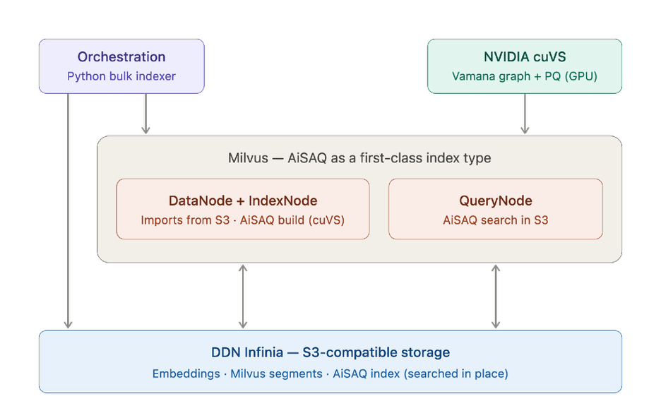
Why the index build had to move to GPUs
Summary of the architectural components and their purpose:
| Architectural component | Purpose | Motivation |
| NVIDIA cuVS (GPU index build) | Builds the Vamana graph on GPU and serializes it in DiskANN-compatible format | Graph construction is dominated by distance computations — days at billion-vector scale on CPU. Prior published results measured a 20× build-time reduction (28.4 → 1.4 days at 4.8B on four H100s, 7.8× end-to-end); IBM Research reported four days on six NVIDIA H200s for 100B vectors vs. an estimated 120 days on CPU |
| AiSAQ post-processing | Converts the cuVS output into the all-in-storage index layout | Decouples index capacity from server DRAM so the index lives entirely in storage |
| Host-core search | Executes ANN search on CPUs against the storage-resident index | Keeps GPUs dedicated to the index build phase; query serving needs no GPU footprint |
Benchmark setup
| Item | As tested |
| Dataset | 1 billion (960 million) x 1,024-dimension fp32 embeddings, Falcon dataset, 3.9 TB raw |
| Build and query node | 8 x NVIDIA H100, 224 vCPU, 2,015 GB DRAM; the AiSAQ search path holds under 1 GB of host memory (indexing runs on the GPUs) |
| Milvus | Milvus 3.0 with cuVS-accelerated AiSAQ indexing; 8 index nodes, 8 data nodes |
| DDN Infinia | Infinia 2.4, 10 storage nodes and one client node; S3 interface |
| Network | NVIDIA ConnectX-8, each NIC using two ports at 400 Gb/s per port |
| AiSAQ | Scale layout; max_degree 64, search_list_size 256, inline_pq 0, rearrange true, num_entry_points 1000 (the same graph parameters as KIOXIA’s prior published 4.8-billion single-server run) |
| Software | NVIDIA cuVS on CUDA 12.9.1; search driven by a custom benchmark script; concurrency 1, 2, 4, 8, 16 clients; batch size 1 |
| Phases | Upload, bulk import, clustering compaction, AiSAQ index build, load and search, each measured separately |
Index Build Results
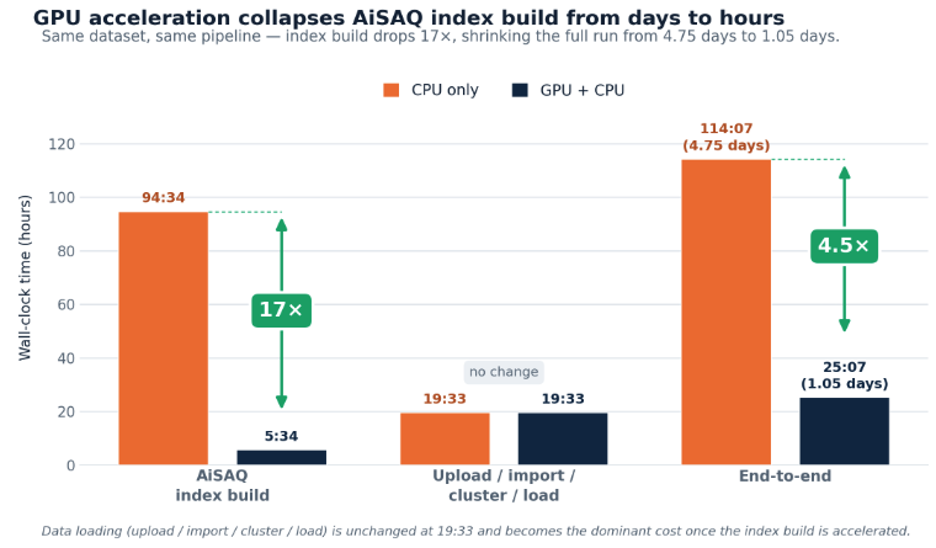
We report the index-build acceleration and the end-to-end acceleration as two separate numbers, because they answer different questions and the gap between them is itself informative: once the graph build is accelerated, un-accelerated data movement becomes the dominant issue.
Search Results
Search, 1B × 1024D, index resident on Infinia
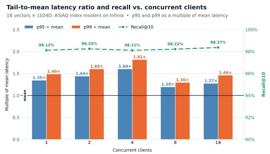
Every result above pairs latency with recall. A latency number without a recall number isn’t a result, because you can always go faster by using lower recall and skipping valuable information. Recall@10 holds at about 98% across every concurrency level, so all latencies are measured at the same quality bar.
We report p99 as well as p95 because retrieval sits on the critical path. It runs in full before the LLM produces its first token, and agentic workflows repeat it at every retrieval hop. A low mean latency doesn’t show the actual user experience if tail latency is high. A tail that looks small per query compounds – across five sequential hops, roughly 1 in 20 requests will hit at least one p99-slow retrieval.
The tail is tight. At every load level from 1 to 16 concurrent clients, p99 stays within 1.3–1.8× of mean latency, and p95 within 1.2–1.6×. Latency rises with load, but the spread around the mean doesn’t blow out and even requests hitting the p95 or p99 latency are returned quickly. To our knowledge, this is the first AiSAQ result to report p99.
Small-Read Latency Matters More Than Bandwidth. A query is a dependency chain where each hop’s address is known only after the previous read returns. The storage must deliver a high rate of small reads with low latency at the p99, under concurrent load because it cannot pipeline the reads. For this reason, not every S3-compatible distributed store works well here. A throughput-tuned object store can post excellent GB/s and still perform badly on this workload because every read sits on the critical path. This workload needs storage built from the ground up for minimizing small-object latency.
What this changes
Capacity stops being a per-server property. Index size and query throughput scale on separate axes. Adding query capacity does not mean copying the index.
Freshness becomes a business cadence. GPU-accelerated builds turn a multi-day reindex into something that fits inside a maintenance window.
The economics invert. Index capacity is priced against flash storage, not DRAM — and against shared flash storage, so it is not stranded.
It is a complete pipeline, not a component benchmark. Ingestion, build, load and search on one architecture, with every phase reported separately.
What’s next
We are aiming for extreme scale —100B and 1Trillion vectors, with more GPUs and higher embedding dimensions. We see value in deeper GPU integration in the retrieval path as NVIDIA cuVS continues to push the boundaries on what’s possible. Finally, we would like to publish a full reference architecture including reproduction steps.